A Deeper Dive Into Graphs
A few months ago, I published a story about the difference between graphs and trees titled “Graphs vs. Trees: The Short Story”. Today, I wish to continue the storyline by taking a closer look at graphs as a whole. While we will still be looking at the bigger picture of things, the following should give a much greater insight into graphs than what was given last time.
To quickly review, the main point in the previous story was that graphs are basically just unordered trees. This was mainly referring to an undirected and unweighted graph. If a graph is directed, weighted, or both, the statement still stands except there now exist a slightly more nuanced definition of “unordered”.
Directed Graphs
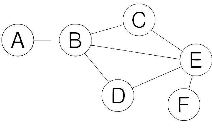
Let’s start with directed graphs. First, take a look at an undirected graph below:

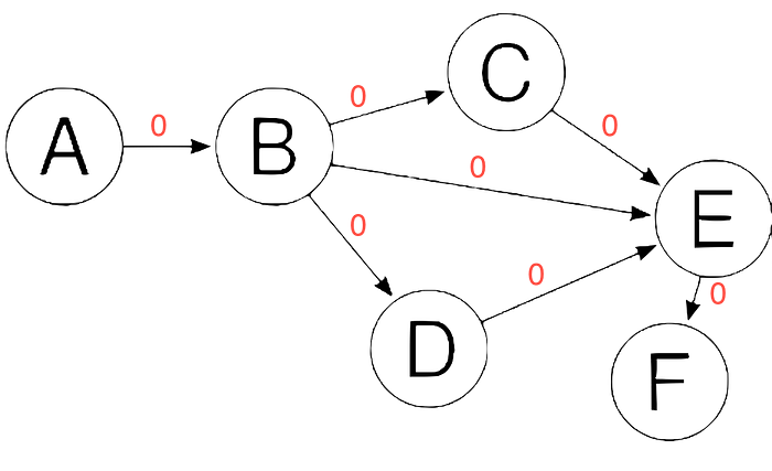
With an undirected graph, you are free to move between vertices in any order that you can come up with. Now, look at a directed version of the graph:

This is where things change. You may only move between vertices in the direction of the arrow attached to each edge. For example, you could move from A to B, but not from B to A. A little more restrictive, right?
Weighted Graphs
Now let’s consider adding weight to our edges. First, imagine that each edge on the graph has a price; a price that has to be paid if one wants to cross the edge. For now, imagine that all edges have the price of zero (free).

This does not really change much, as there was no price to pay to begin with. We can still traverse the graph without thought, as long as we abide by the direction of the arrows. Even if each edge has a price, as long as they all are the same amount, it still does not matter for every edge has the same importance, or weight.

Okay, but what if the prices were different? How would that change the way we traverse the graph?

Since the prices are now different from each other, a new dynamic is introduced. Going from vertex to vertex now costs different amounts of “money”. Sometimes there is only one path to take, but other times, one can chose which way they want to go next, with the price usually serving as a factor in that decision. In general, when going from one vertex to another somewhere else on the graph, the “cheapest” path is the desired one. For example, if I wanted to take the cheapest route from A to E, I would go ABDE. Although an initial reaction might be to just go ABE, this path actually cost more. Adding everything up, the cost of ABE is eleven while ABDE is only nine. This is the basic concept of weighted graphs.
Up until this point, I have referred to the numbers representing each edge as its “price”, in reference to money. In reality, the numbers are actually referred to as an edge’s “weight” (hence the name of the topic). Introducing everything through the analogy of money can be an easier first approach as money is a concept that most of us are familiar with. There are other ways to think about this, as well. You could imagine the numbers as the distance between the two vertices. Most illustrations of graphs wouldn’t be to scale with this thinking, but it’s a valid analogy nonetheless.
Representing Graphs in Code
Alright, we now have a good understanding of what directed and weighted graphs are, but how do we even represent graphs in code? We have only been using illustrations of graphs thus far. Well, it turns out that there are numerous ways of representing such. Let’s explore a few. The code examples for each method will be referring to the directed and unweighted example graph shown previously.
Edge List
An edge list is exactly what it sounds like; a list of all the edges in the graph. Keep in mind that an edge is represented by its start and end vertex.

Adjacency List
An adjacency list is simply a dictionary with each key being a vertex in the graph, and each value being everything that that vertex is adjacent to. With a directed graph, the arrows have to be pointing in the proper direction for a vertex to be on the list.

Adjacency Matrix
The adjacency matrix is often better understood if it is first represented as a drawing. If you have experience with matrices in calculus, then this should come pretty easy to you. If not there is no need to worry, just take it one step at a time.

With an adjacency matrix, a “0” means that the two vertices are not adjacent, and a “1” means that they are. There is a mountain of ways to manipulate and work with a matrix, but that is out of scope for this explanation. Notice how there are only zeros on the diagonal. Think about why this would be the case…
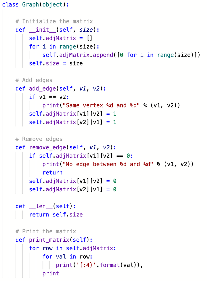
As far as coding an adjacency matrix goes, there are multiple ways to go about it. The following uses OOP:

When To Use Each Method
Each method is a valid representation of a graph, so when should you use one over the other? The short answer is that it really depends on what you are doing and how you wish to manipulate the data. For example, an adjacency matrix is great and easy to use, but can take up much more memory in comparison to say an edge list. Also note that each method is fully capable of containing an edge’s weight if it was a weighted graph; this information was left off of the examples for simplicity purposes.
In Conclusion
The world of graphs in computer science is vast, and while this is only scratching the surface, you should hopefully now have a better understanding of the basics moving forward.
To further the understanding of graphs, I encourage looking into traversal algorithms, like DFS (Depth-First Search) and BFS (Breadth-First Search).
BFS, geeksforgeeks.org
DFS, geeksforgeeks.org